
In this article, I will walk you through everything you need to know about PARTITION BY. We will cover its internal architecture, how it compares directly to GROUP BY, its primary syntax patterns, advanced framing techniques, performance optimization strategies, and common pitfalls to avoid.
SQL PARTITION BY
What Is the SQL PARTITION BY Clause?
The PARTITION BY clause is a sub-clause of the OVER() clause used in SQL window functions. It divides a query’s result set into discrete, isolated partitions—or logical subsets—based on the values of one or more specified columns.
Once the data is split into these logical windows, the specified window function (such as SUM(), AVG(), or ROW_NUMBER()) performs its computation independently across the rows inside each partition.
SQL
<window_function>() OVER (
    PARTITION BY column1, column2, ...
    ORDER BY column3 [ASC|DESC]
)
Key Architectural Characteristics
- Preservation of Row Identity: Unlike standard grouping operations,
PARTITION BYdoes not collapse multiple input rows into a single summary row. Every original row from theFROMandWHEREclauses remains in the final output. - Independent Window Scope: Each partition acts as an isolated boundaries for the calculation. When the window function reaches the end of a partition, its internal state (like a running sum or row counter) resets before moving to the next partition.
- Multi-Column Partitioning: You can partition by a single column (e.g.,
department_id) or a composite set of columns (e.g.,state, city, store_id) to create multi-tier analytical subsets.
PARTITION BY vs. GROUP BY: Understanding the Core Difference
One of the most frequent points of confusion among mid-level database engineers is knowing when to use GROUP BY versus PARTITION BY.
GROUP BYcollapses rows sharing the same key into a single summary row per group. If you need a high-level executive dashboard showing total quarterly revenue by region,GROUP BYis the right choice.PARTITION BYretains every single underlying row while attaching calculated partition-level metrics as additional columns. If you need to list every employee alongside their individual salary and their department’s average salary,PARTITION BYis required.
Structural Comparison Table
| Dimension | GROUP BY Clause | PARTITION BY Clause |
| Output Row Count | Reduces row count (1 row per group) | Preserves original row count |
| Context Scope | Query-wide aggregation | Row-level window context |
| Syntax Location | Standalone query clause after WHERE | Placed inside the OVER() clause |
| Select List Restriction | Unaggregated columns must be in GROUP BY | Any column from the source table can be selected |
| Primary Use Cases | High-level summary reports, KPI rollups | Running totals, rankings, moving averages, deduplication |
Essential Window Functions That Utilize PARTITION BY
To leverage PARTITION BY effectively, you must pair it with the appropriate window function. Window functions generally fall into three distinct categories:
1. Ranking Functions
Ranking functions evaluate the position of a row within its partition based on a specified ordering.
ROW_NUMBER(): Assigns a unique, sequential integer to each row within the partition, starting at 1. Ties receive distinct numbers arbitrarily unless secondary order columns are defined.RANK(): Assigns a rank to each row based on theORDER BYcriteria. Rows with identical values receive the same rank, but subsequent rank values are skipped (e.g., 1, 2, 2, 4).DENSE_RANK(): Similar toRANK(), but does not skip rank values when ties occur (e.g., 1, 2, 2, 3).NTILE(n): Divides the rows within each partition intonroughly equal buckets and assigns the bucket number (1 throughn) to each row.
2. Aggregate Functions
Standard aggregate functions can be transformed into window functions by adding an OVER(PARTITION BY ...) clause.
SUM(): Calculates the cumulative total or partition total.AVG(): Calculates the average value across the partition.COUNT(): Counts the number of non-null records within the partition.MIN()/MAX(): Identifies the minimum or maximum scalar value within the partition.
3. Navigation & Value Functions
Navigation functions let you inspect values from other rows in the partition relative to the current row without performing explicit self-joins.
LAG(column, offset): Accesses data from a previous row at a specified offset within the partition.LEAD(column, offset): Accesses data from a subsequent row at a specified offset within the partition.FIRST_VALUE(column): Returns the first value in the partition frame according to the ordering.LAST_VALUE(column): Returns the last value in the partition frame according to the ordering.
Core SQL Patterns & Usage Scenarios
Let’s explore three critical design patterns where PARTITION BY proves indispensable in real-world database architecture.
Pattern 1: De-Duplication Using ROW_NUMBER()
In operational databases, duplicate events or staging records frequently occur due to network retries or batch ingestion overlaps. To clean up a dataset while retaining the latest record per entity, we partition by the natural business key and order by the timestamp in descending order.
SQL
WITH RankedCustomerUpdates AS (
    SELECT
        customer_id,
        first_name,
        last_name,
        email,
        state,
        updated_at,
        ROW_NUMBER() OVER (
            PARTITION BY customer_id
            ORDER BY updated_at DESC
        ) AS row_num
    FROM staging_customer_feed
)
SELECT
    customer_id,
    first_name,
    last_name,
    email,
    state,
    updated_at
FROM RankedCustomerUpdates
WHERE row_num = 1;
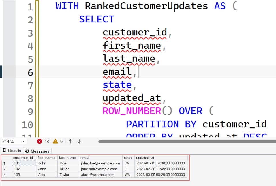
After executing the above query, I got the expected output as shown in the screenshot below.
How It Works:
The query partitions data by customer_id. Inside each customer’s partition, rows are ordered so that the newest updated_at record receives row_num = 1. Filtering for row_num = 1 cleanly isolates the authoritative record for every customer.
Pattern 2: Contextual Metrics (Row Value vs. Partition Average)
Suppose our HR team needs a report listing every employee’s salary alongside their department’s average salary, as well as the variance between their salary and that departmental benchmark.
SQL
SELECT
    employee_id,
    full_name,
    department_name,
    office_location,
    salary_usd,
    AVG(salary_usd) OVER (
        PARTITION BY department_name
    ) AS dept_avg_salary,
    salary_usd - AVG(salary_usd) OVER (
        PARTITION BY department_name
    ) AS variance_from_avg
FROM US_Employees
ORDER BY department_name, salary_usd DESC;
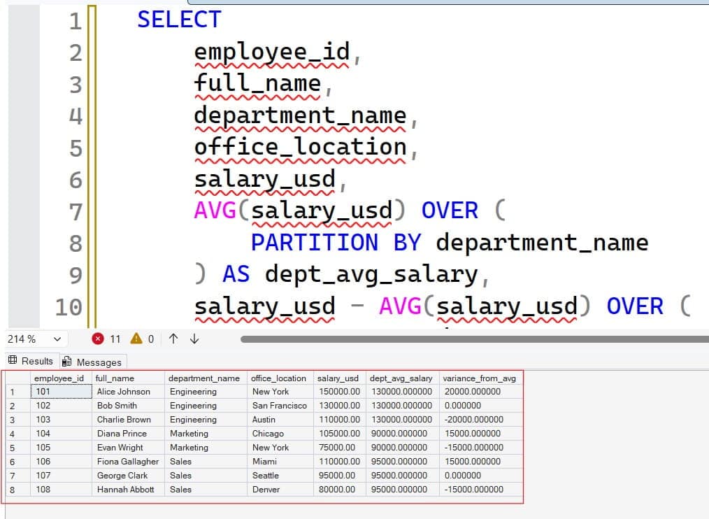
After executing the above query, I got the expected output as shown in the screenshot below.
How It Works:
The AVG(salary_usd) OVER (PARTITION BY department_name) computes the mean compensation specifically for the employee’s department. Because row identity is preserved, we can subtract the windowed average directly from the row’s salary_usd scalar value in the same query pass.
Pattern 3: Calculating Running Totals by Partition
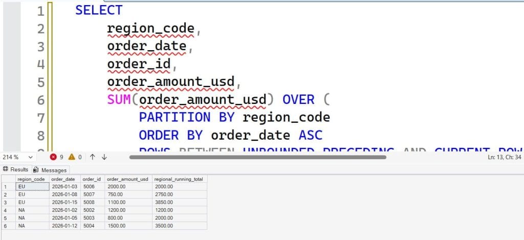
Tracking year-to-date sales per region requires calculating a cumulative sum that accumulates sequentially within each region and resets at regional boundaries.
SQL
SELECT
    region_code,
    order_date,
    order_id,
    order_amount_usd,
    SUM(order_amount_usd) OVER (
        PARTITION BY region_code
        ORDER BY order_date ASC
        ROWS BETWEEN UNBOUNDED PRECEDING AND CURRENT ROW
    ) AS regional_running_total
FROM sales_orders
WHERE order_date >= '2026-01-01'
ORDER BY region_code, order_date;
After executing the above query, I got the expected output as shown in the screenshot below.
Advanced Window Framing: ROWS vs. RANGE
When an ORDER BY clause is included within an OVER() window containing PARTITION BY, SQL applies a default window frame specification. Understanding window framing allows you to fine-tune exactly which rows within the partition are included in the window calculation.
Syntax Structure
SQL
{ ROWS | RANGE } BETWEEN frame_start AND frame_endCommon frame boundary specifiers include:
UNBOUNDED PRECEDING: Starts at the very first row of the partition.n PRECEDING: Looks backnrows prior to the current row.CURRENT ROW: Limits the frame to the current evaluation row.n FOLLOWING: Extends forwardnrows after the current row.UNBOUNDED FOLLOWING: Extends to the very last row of the partition.
ROWS vs. RANGE: The Critical Difference
ROWSoperates on physical row offsets regardless of duplicate values in the ordering column.RANGEoperates on logical value ranges in the ordering column. If multiple rows share the exact same order value (a tie),RANGEtreats all tied rows as a single group, including all of them in the window frame simultaneously.
Architectural Tips: Always default to
ROWS BETWEEN ...when calculating cumulative totals or moving averages. In engines like PostgreSQL and SQL Server,ROWSavoids the heavy temporary spooling and sorting overhead associated with evaluating logical ties underRANGE.
Performance Optimization & Indexing Strategies
While PARTITION BY provides massive expressive power, executing window functions across multi-million row datasets can lead to CPU spikes and memory exhaustion if improperly indexed.
The POC Indexing Rule
To optimize queries using PARTITION BY ... ORDER BY, structure your composite indexes using the POC Pattern:
- P – Partition: Place the
PARTITION BYcolumn(s) first in the index key definition. - O – Order: Place the
ORDER BYcolumn(s) second in the index key definition. - C – Cover: Include any remaining query projections (columns in
SELECT) asINCLUDEcolumns (in SQL Server/PostgreSQL) to avoid key lookups.
Example Index Definition:
SQL
-- Query:
-- OVER (PARTITION BY store_id ORDER BY transaction_timestamp DESC)

-- Optimal Composite Index (PostgreSQL Syntax):
CREATE INDEX idx_transactions_poc
ON store_transactions (store_id, transaction_timestamp DESC)
INCLUDE (amount_usd, customer_id);
Why the POC Pattern Works
When the database query planner finds a matching POC index, it can stream data directly from index leaf pages in pre-partitioned and pre-sorted order. This eliminates the need for expensive explicit SORT or HASH MATCH operations in memory or on disk (tempdb / disk spools).
Common Pitfalls & Best Practices
A few common implementation mistakes:
1. Confusing Query Partitioning with Table Partitioning
Query-level window partitioning (PARTITION BY in OVER()) is entirely distinct from database table partitioning (such as range partitioning a large table by month on disk). Query partitioning is a runtime data grouping mechanism within memory, whereas table partitioning is a physical storage architecture.
2. Attempting to Filter Window Functions in WHERE Clauses
Window functions are evaluated after WHERE, GROUP BY, and HAVING clauses during logical SQL execution order. Consequently, you cannot use window functions directly in a WHERE clause:
SQL
-- ❌ INVALID SQL: This will cause a compilation error
SELECT employee_id, salary_usd
FROM US_Employees
WHERE ROW_NUMBER() OVER (PARTITION BY department_id ORDER BY salary_usd DESC) = 1;
Correct Fix: Wrap the window function inside a Common Table Expression (CTE) or derived table subquery, then filter the calculated column outside.
SQL
-- ✅ VALID SQL: Using CTE for logical separation
WITH RankedEmployees AS (
    SELECT employee_id, salary_usd,
           ROW_NUMBER() OVER (PARTITION BY department_id ORDER BY salary_usd DESC) AS rank_num
    FROM US_Employees
)
SELECT employee_id, salary_usd
FROM RankedEmployees
WHERE rank_num = 1;
3. Redundant Window Specifications
If your query contains multiple window functions that share the exact same PARTITION BY and ORDER BY definitions, write clean, dry code by taking advantage of named windows (where supported by your engine, such as PostgreSQL or MySQL 8.0+):
SQL
SELECT
    employee_id,
    department_id,
    salary_usd,
    SUM(salary_usd) OVER w AS dept_total_salary,
    AVG(salary_usd) OVER w AS dept_avg_salary,
    COUNT(employee_id) OVER w AS dept_headcount
FROM US_Employees
WINDOW w AS (PARTITION BY department_id);
Summary & Key Takeaways
Mastering PARTITION BY elevates your SQL capabilities from writing basic data extraction scripts to constructing highly sophisticated, enterprise-grade analytical queries.
- Use
GROUP BYwhen you need aggregated summary datasets with a reduced row count. - Use
PARTITION BYinsideOVER()when you need contextual metrics, running totals, or ranking calculations while preserving every underlying row. - Pair
PARTITION BYwith the POC indexing strategy (PartitionKey,OrderKey) to optimize production query performance.
You may also like the following articles:

After working for more than 15 years in the Software field, especially in Microsoft technologies, I have decided to share my expert knowledge of SQL Server. Check out all the SQL Server and related database tutorials I have shared here. Most of the readers are from countries like the United States of America, the United Kingdom, New Zealand, Australia, Canada, etc. I am also a Microsoft MVP. Check out more here.